This code was made for the final project of a computational physics class at UCLA. It was my introduction to computational plasma physics.
All of the code is on my github, along with more detailed explanations and code tests in the jupyter notebook.
The full animation is at the bottom of the page.
what is particle in cell?
Particle in cell (PIC) is a method to simulate the movement of particles under a force of some kind, which in my case is the force from an electric field, essentially simulating a plasma. At it’s core, a (1D) PIC code uses a mesh grid that has bins/cells. The edges of these bins are described by two $x$ coordinates, $x_j$ and $x_{j+1}$ (of course, in 2D or 3D, there’s more coords), and within that bin is a particle $i$ with location $r_i$. And from these particle locations, a denisty can be calculated at the edges as
$$ \rho_j = \sum_{i=0}^{N_p}\frac{x_{j+1} - r_i}{\Delta x}, \quad \rho_{j+1}=\sum_{i=0}^{N_p}\frac{r_i - x_{j}}{\Delta x}, $$
where $N_p$ is the number of particles within a bin and $\Delta x$ is the length of the cell. The particle in cell code that I made is the simplest case possible (I say that but it was very difficult and I needed a lot of guidance from my TA), as in it is 1D and electrostatic (time-independent) such that Maxwell’s equations are
$$ \nabla \cdot E = \rho, \quad \nabla \cdot B = 0 \\ \nabla \times E = 0, \quad \nabla \times B = 0. $$
We ultimately want to find the acceleration
$$ F = ma = -qE \\ \implies a = -\frac{q}{m}E = -\frac{q}{m}\frac{\text{d}\phi}{\text{d}x}, $$
as that is what pushes the particles. $\phi$ is found through combining the $E$ maxwell equations, such that
\begin{equation} \frac{\text{d}^2\phi}{\text{d}x^2} = \rho \qquad \text{poisson’s equation}. \end{equation}
And from acceleration, we can find velocity and position, giving us our phase space.
solving methods
Poisson’s equation can be estimated using the finite difference method so I tried that first. The first derivative of a general function using the finite difference method yields
$$ f’(a) = \frac{f(a+h)-f(a)}{h}, $$
so then
$$ f’’(a) = \frac{f(a) - 2f(a+h) + f(a+2h)}{h^2}. $$
If we apply this function to our $\phi$, we can define $f(a+h)$ as $\phi_j$, so then from equation $1$,
$$ \frac{\text{d}^2\phi}{\text{d}x^2} = \frac{\phi_{j-1} - 2\phi_j + \phi_{j+1}}{\Delta x^2}=\rho. $$ But using the matrix that comes from this finite difference equation doesn’t get us anywhere because it’s not invertible :( …. so we will use a method involving a discrete fourier transform instead. According to Birdsall, we know that $$ \phi(k) = \frac{\rho(k)}{k^2} \quad \text{and} \quad k = \frac{2n\pi}{L}, $$ where $\rho(k)$ is our charge density. To transform to $\rho(k)$, we use
$$ G(k) = \Delta x \sum_{j=0}^N{G(x_j)} e^{-ikx_j} $$ and to transform back to $\phi(x)$, we use the inverse DFT $$ G(x_j) = \frac{1}{L} \sum_{n=-N/2}^{N/2}{G(k)} e^{ikx_j}. $$
Using $\phi$, we can now find $E$. Since we are only looking at the electric field from bin to bin in the mesh, we can approximate it as just the slope between two points, $\phi_{j-1}$ and $\phi_{j+1}$, such that
$$ E_j = \frac{\text{d}\phi(x_j)}{\text{d}x} = \frac{\phi_{j+1} - \phi_{j-1}}{2 \Delta x}, $$
which is represented in matrix form as
$$ E = \frac{1}{{2 \Delta x}} \begin{pmatrix} 0 & 1 & 0 & \dots & 0 & -1 \\ -1 & 0 & 1 & & & 0\\ 0 & -1 & 0 & & & \vdots\\ \vdots & & & \ddots & & 0\\ 0 & & & -1 & & 1\\ 1 & 0 & \dots& 0 & -1 & 0 \end{pmatrix} $$
We want the electric field at the locations of the particles within a bin at $r_i$. Thus, we essentially take a weighted average of the electric fields at $E_j$ and $E_{j+1}$ with weights used earlier to get the total electric field at $r_i$, such that
$$ E_i = \frac{x_{j+1} - r_i}{\Delta x} E_j + \frac{r_i - x_{j}}{\Delta x} E_{j+1}, $$
which is what we plug back in to our original acceleration. We repeat this process until a time $t_{final}$.
plasma background
To produce something like a two stream instability with my PIC code, I first had to understand some plasma basics.
fundamental equations
The essential plasma equations are
\begin{align} \text{Vlaslov} \quad &\partial_t v + v\partial_x v = -\frac{e}{m} E \\ \text{continuity} \quad &\partial_t n + \partial_x(n v) = 0 \\ \text{Gauss} \quad &\partial_x E = -\frac{e}{\epsilon_0}(n - n_0) \end{align}
plasma oscillations
For plasma oscillations, $n, v$ and $E$ are described by a constant background and a perturbation indicated by a $0$ and $1$ index, respectively, such that
\begin{align} n &= n_0 + n_1 \\ v &= v_0 + v_1 \\ E &= E_0 + E_1. \end{align} If we look at the continuity equation and plug in $n$ and $v$, we see that
$$ \partial_t (n_0 + n_1) + \partial_x((n_0 + n_1)(v_0 + v_1)) = 0, $$
where $\partial_t n_0$ and $\partial_x(n_0v_0)$ go to zero because $n_0$ and $v_0$ are constant over time. Then after algebra,
$$ \partial_t n_1 + \partial_x(n_1v_0 + n_0v_1 + n_1v_1) = 0. $$
And taking second order terms to be zero,
$$ \partial_t n_1 + \partial_x(n_1v_0 + n_0v_1) = 0. $$
We can analyze two cases: no drift velocity ($v_0 = 0, E_0 = 0$) and yes drift velocity ($v_0 \neq 0$). For each case, the continuity equation becomes
\begin{align} \text{no drift} \quad &\partial_t n_1 + n_0\partial_x v_1 = 0 \notag \\ \text{ya drift} \quad &\partial_t n_1 + \partial_x n_1v_0 + n_0\partial_x v_1 = 0. \notag \end{align}
Then, for a plane wave $f_1(x, t)$ of amplitude $f_1$, we obtain
$$ -i \omega n_1 + i k n_0 v_1 = 0. $$
This process is done for all 3 equations in $(2), (3)$ and $(4)$, so we end up with 2 sets of 3 equations, which leads to the results of
\begin{align} \left(1 - \frac{\omega_p^2}{\omega^2}\right)E_1=0 \qquad &\text{Dispersion relation} \ (v=0) \notag \\ \left(1 - \frac{\omega_p^2}{(\omega-kv_0)^2}\right)E_1=0 \qquad &\text{Doppler waves} \ (v\neq0) \notag \end{align}
These relations are useful because they relate $k$ and $\omega$ of a given wave.
two stream instability
In two stream instability, there are two populations of particles with densities $n_{0_1}$ and $n_{0_2}$, such that $n_0 = n_{0_1} + n_{0_2}$. There is also a constant background of ions that do not move through out the simulation such that the plasma is quasi-neutral. Since these ions are immobile, they essentially have an infinite mass. Additionaly, $v_{0_1} = 0$ and $v_{0_2} = v_0 \neq 0$. If we apply these conditions to $(2), (3)$ and $(4)$, we find that
\begin{align} &\partial_t v_i + v_i \partial_x v_i = -\frac{e}{m} E \notag \\ &\partial_t n_i + \partial_x(n_i v_i) = 0 \notag \\ &\partial_x E = -\frac{e}{\epsilon_0}(n_1 + n_2 - n_0), \notag \end{align}
Following the same process we did for plasma oscillations, we end up with
\begin{gather} \left[1 - \frac{\omega_p}{\omega^2} + \frac{\omega_p}{\omega-kv_0}\right]E_1 = 0 \notag \\ \implies 1 - \frac{\omega_{p_1}^2}{(\omega-kv_{0_1})^2} - \frac{\omega_{p_2}^2}{(\omega-kv_{0_2})^2} = 0 \notag \end{gather}
which means that when $\omega_{p_1}=\omega_{p_2}=\omega_{p_e}$ and $v_{0_1}=-v_{0_2}=v_0$,
$$ 1 = \frac{1}{\hat{\omega} - \alpha} + \frac{1}{\hat{\omega} + \alpha}, $$
where
$$ \omega_p = \frac{n_0 e^2}{\epsilon_0m}, \qquad \hat{\omega} = \frac{\omega}{\omega_p}, \qquad \alpha = \frac{kv_0}{\omega_p}. $$
And as the phase space shows, unstable modes appear in the plasma, even with low temperatures. The fastest growing mode $k_{max}$ is found by maximizing $\hat{\omega}$ with respect to $\alpha$, such that
\begin{gather} \frac{\text{d}\hat{\omega}}{\text{d}\alpha} = 0 \implies \alpha = \frac{\sqrt{3}}{2}\frac{k_{max}v_0}{\omega_{p_e}} \notag \\ \implies k_{max} = \frac{\sqrt{3}}{2}\frac{\omega_{p_e}}{v_0}. \notag \end{gather}
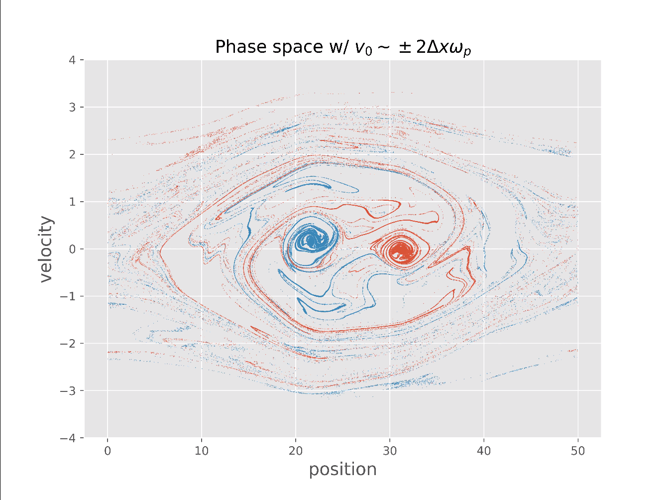
And the fastest growing mode corresponds to the number of phase space holes. At $v_0\simeq \pm 10 \Delta x \omega_{p_e}$, there should be one phase space hole, while at $v_0\simeq \pm 2\Delta x \omega_{p_e}$, there should be many phase space holes.
results — two stream instability
This is an example of two stream instability with my PIC code (it goes quite fast so feel free to slow it down or click through it):
There’s a couple problems with the results. One being that the animation is quite rigid and squarish. Maybe something to do with my solver?
The other problem being the amount of phase space holes. With $v_0\simeq \pm 2 \Delta x \omega_{p_e}$, I would expect more than just two holes, while with $v_0\simeq \pm 10 \Delta x \omega_{p_e}$ (not here), I would expect only one, but I also get two holes. To solve this, I think I would have to dig into the physics more.